Updated Book Club Planning

I run a book club called Women, Wine, and Crime in the Denver, CO area, open to women interested in murder mystery and true crime books. I took over this book club in August of 2020, we read fiction and non-fiction, a new book every (roughly) 6 weeks. I find that six weeks, along with some other parameters I’ve fine-tuned, has increased attendance and more members have fished a larger portion of the book. Here’s a list of past, present, and potential books we’ve read.

I started doing a book every 6 weeks or so last year and it really improved attendance; people had more time to read and more fodder for conversation. We go to different places each time and I initially hadn’t kept track. A few favorites are now closed and I’ve been getting more recommendations from members so I started a sheet that has locations, if they’re good, need to be re-vetted, or are a “no” with qulifiers of “closed” or “bad”; bad being either rudeness, group size difficulties, or parking issues.

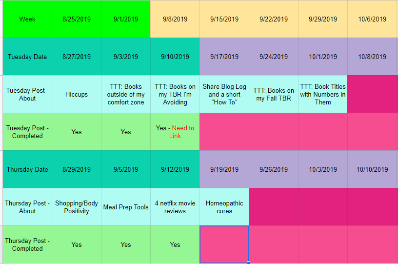
I’ve made some changes and have explanded my GoogleSheets that I use plan and organize upcoming events and books.
^{“my GoogleSheets” is a hyperlink to the actual organizer for you to check out as inspo}

Recently, memebers have been asking me for more events that are not necessarily book reviews. I’ve decided to comply with the masses and, sandwiched between evey other book, add some other activities. Since the book club is named Women, Wine, and Crime, I decided that the first two would be No Crime, Just Wine; just to get together. The third one will be a book exchange in July since the one in December went well. Essentially, it’s scheduled: book, six weeks, book, three weeks, event, three weeks, book, six weeks, book, etc. So we don’t have an event every three weeks which I think would run the members ragged. The first No Crime, Just Wine, is January 27th; I’ll let you guys know how it goes!

If you view the sheets, let me know if you have any recommendations to improve. I’m also always looking for book recommendations, for the book club or otherwise. If you run a book club, I hope this helps.

*If you enjoyed any part of this post, please consider liking it. If you loved it, please consider following me on WordPress. I also love comments including questions, advice, or a review of the post itself. Thank you for reading and best of luck in your adventures.*

My New Fav Blogging Tool

Hint: it’s a Google Sheets conditionally formatted log and I’m gonna show you mine and help you make yours!

Mine

Quick brief explanation:
Row 1: My "calendar" is built of Sun-Sat weeks because my work schedule goes Sun-Sat. The "Week" the the Sunday that heads that week up.

Row 2: Tuesday Date is the date of the Tuesday of that week so I stay on track for a TTT post or for a substitute short post.

Row 3: Tuesday Post - About is what the post will be about. Either a general idea or a title.

Row 4: Tuesday Post Completed - Is it done? (Blank means no...)

Row 5: Thursday Date is the date of the Thursday of that week so I have a target date.

Row 6: Thursday Post - About is what the post will be about. Either a general idea or a title.

Row 7: Thursday Post Completed - Is it done? (Blank means no...) 

I know that got a little repetitive, it was important to do so. For mine:::
When the “about” rows are filled, they go from pink to bluish teal.
When they “completed” rows have data, they go from pink to green.
When the “completed” rows have data, their corresponding date turn teal so I know the post for that date is done.
When both “completed” rows of a week say “yes” and only “yes”, Row 1’s “date” will turn green to show that the week is completed.

(side note- I decided to switch my homeopathic cures and this posts' post dates... so...)

Pretty nifty, huh? Want one for yourself? Here’s how you get like me.

1. First, figure out whether your week starts on Sunday or Monday.
2. Open a new GoogleSheets doc, name it something fun and exciting like “blog log” or “dinosaur dreams”.
3. Consider your color spectrum, you’ll need two. One for when items are not complete and one for when they are. I went with yellow pink and purple for my “incompletes” and shades of green for my done done done.
4. Row One
   1. Title the first cell
   2. In the next two cells type in the first two “start of the week” dates.
   3. Click and hold your mouse over A:1 and drag the mouse over the rest of the row, it’ll repeat the pattern you created.
   4. Click the “1” so it highlights the row, pick your “head of the week incomplete” color.
5. Row Two
   1. Repeat steps one and two of Row One, but with the date of the week for the days of your first weekly blog post
      (Two Monday dates, or whatever you do boo boo).
   2. Click the “2”, choose your “incomplete” color
6. Row Three
   1. Title the first cell
   2. Click the “3” and choose your “incomplete” color
7. Row Four
   1. Title the first cell
   2. Click the “4” and choose your “incomplete” color
8. Rows Five Through Seven
   1. Repeat Rows Two through Four.
9. If you do more than two regular posts a week, repeat as needed for your days of the week.

Whew! Now your “incomplete” is set and you’re ready for some conditional formatting.

1. Row One
   1. =And($B$4:$Z$4=”yes”, $B$7:$Z$7=”yes”)
      This is the code I have, as you can see it uses a conditional formula which is dependent upon Row 4 (B4 through Z4, and Z is my current last column) equaling “yes” as well as a conditional for Row 7 set the same way. If you are going to have more than the two posts, be sure to extend the conditions. My Row 4 and Row 7 are the two rows where my “post completed”s are. So once both posts for the week are completed, with no contingencies, and the cells say “yes” and only “yes”, the week is done. (the “=” is part of the equation)
   2. Once the formula is set, select the color for the condition. In the same side-bar that the column is written there’s a color selection. It should have auto-populate with the “incomplete” color you chose so be sure to change it to what you would like as your “complete” color.
2. Row Two
   1. =$B$4:$Z$4>0
      This formula references Row 4 (where my “post completed” for that day is) only and the “>0” is greater-than-zero meaning as long as there is a value row four of the same column, the formatting applies.
   2. Pick the color for this formula being complete
3. Row Three
   1. Since this row is conditional only upon itself you just click the cell, select conditional formatting, and when the side bar comes up there is a drop down. From the drop down choose “is not empty” and
   2. Pick your “completed” color
4. Row Four
   1. Same as Row Three
5. Row Five
   1. =$B$7:$Z$7>0
      Just like Row Two but referencing Row 7
6. Row Six
   1. Same as Row 3
7. Row Seven
   1. Same as Row 4

And now you’ve got a formatted amazing blog log to help you bloggy blog in the blogosphere!
Get Shwifty!!

Get Shwifty
Rick & Morty S2E5

Got questions? Need help? Comment and I’ll do my darnedest! Happy blogging!

*If you enjoyed any part of this post, please consider liking it. If you loved it, please consider following me on WordPress. I also love comments including questions, advice, or a review of the post itself. Thank you for reading and best of luck in your adventures.*